
Particle shapes
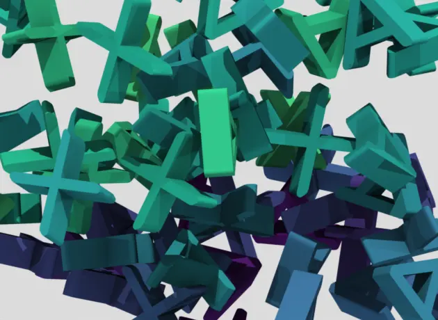
From spheres to superquadrics, and from flexible fibers to arbitrarily shaped particles: Aspherix® offers a wide range of particle shapes to suit every simulation case.
DEM simulations of real materials and processes
A quick overview to sum up the main features and functionalities that make Aspherix® the perfect DEM software for your engineering workflow:
From spheres to superquadrics, and from flexible fibers to arbitrarily shaped particles: Aspherix® offers a wide range of particle shapes to suit every simulation case.
A comprehensive model library covering contact and cohesion, liquid bridges, heat and mass transfer, breakage, wear, electrostatics and more, so that real-world material behavior can be captured directly in Aspherix®.
Everything you need for industrial-scale simulations: coarse-graining, load balancing, GPU support and massive parallelization on CPU HPC clusters.
From particle data and force networks to residence time distributions, collision statistics and spatial averaging: Aspherix® turns simulation results into the numbers that matter for your process.
Dedicated interfaces for connecting Aspherix® to CFD, FEM, multi body dynamics and electric field simulations.
Programmatic access via C++ and Python to extend contact models, add custom equations and access particle and mesh properties.
Watch Aspherix® in action. These six DEM simulations show what particle simulation can do in real engineering work:
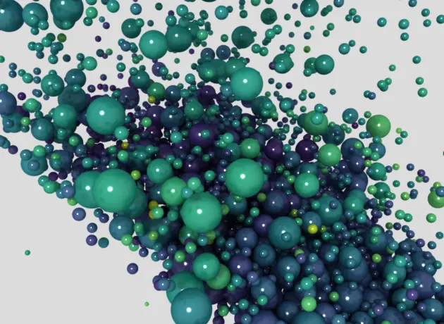
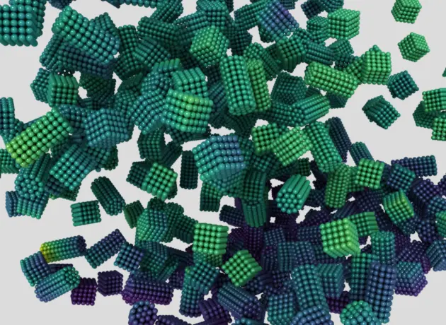
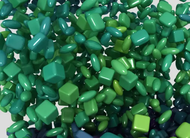
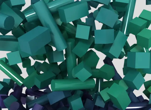
Real particles are rarely round. Aspherix® supports a large variety of particle shapes, so pellets, grains, tablets, ore, fibers or agglomerates can be modelled with the shape that matches the material.
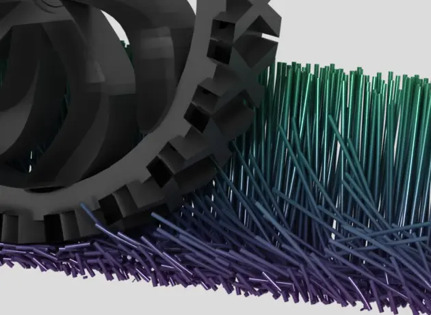
Use spheres, multisperes, superqudrics, convex or concave meshed particles or flexible / breakable agglomerates.
What makes a bulk material behave the way it does happens at the level of individual particles: how particles push, stick, rub and roll against each other, how they take up liquid, exchange heat or break apart. Aspherix® covers these effects with a large library of validated models.
The contact models range from classic Hertz and Hooke formulations to elasto-plastic, adhesive and time- or temperature-dependent variants, with several rolling friction models on top. Cohesive and wet materials are handled by JKR and SJKR cohesion, powder models and liquid bridges that form, transport liquid, evaporate and solidify, from spray coating to agglomeration. Heat conduction, radiation, melting and mass transfer describe thermal and chemical processes, while bond models make it possible to simulate flexible fibers and breakable agglomerates. Attrition and equipment wear show what happens to the product and the machine over time. Electrostatic charging, electrical conductivity and magnetic forces complete the range.
Every model is ready to combine with any other, so the simulation reflects the material, not the limits of the software. Browse the detailed model overview below.
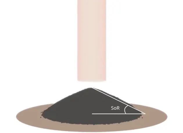
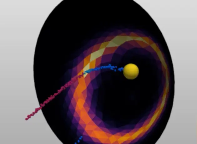
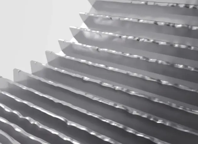
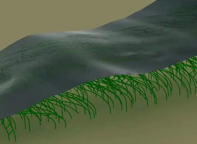
Classical models (Hertz, Hooke, also with time or temperature dependent properties, Thornton-Ning model)
Specialised models for cohesive materials (JKR, Luding, general adhesive elasto-plastic model)
Classic models (including history values, with time and temperature dependent properties)
Specialised models for powder modeling, particle attrition, adhesive materials and bonded particles (Burgers model)
Several elasto-plastic spring models (EPSD)
Constant directional torque (CDT) model as well as a simplistic model from the CDT family (Model A from Ai et al. (2011))
Full & simplified Johnson-Kendall-Roberts (JKR) models, adaptive cohesion model (Obermayr et al. (2014)), cohesion models for powders, asphalt-like materials or cohesively bonded agglomerates
Powder compaction model with options for hardening, elastic dilation, slow compression and the depiction of non linear behaviour
Fibers (bonded particles with no forces / torques between particles), sticky / wet fibers, buckling or plastic deformation of fibers
Parallel bond model (after Potyondy & Cundall (2004)) for modeling flexible agglomerates
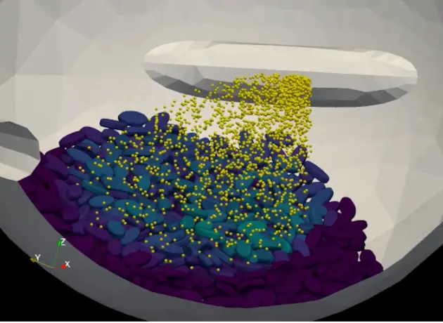
Lagrangian droplets & simplified spray modeling via surface detection
Liquid transport, evaporation, porous particles & sponges
Liquid bridge formation & breakup, solidification of wet agglomerates
Lagrangian bubble model for coalescence & breakup
Multicontact surface model for spherical particles
Plastic powder compression model with options for hardening, elastic dilation, slow compression and the depiction of non linear behaviour
Force-based fragmentation models, deterministic (replacement by set of fragment particles) or according to a fragmentation distribution; resolved and unresolved models (Bruchmueller et al. (2011))
Attrition model for erosive / abrasive particle attrition
Wear models to calculate mesh erosion, abrasion, deformation or a combination thereof (Finnie (1960), Archard (1953), Roessler Katterfeld (2023))
Gravity and models for custom body forces
Drag modeling based on single values, velocity fields or time series of velocity fields
Models to "freeze" particles in certain areas or prescribe predefined velocities
Dedicated sedimentation model for four-way coupled CFD-DEM simulations
Extensive feature set for static and transient one-way coupled CFD-DEM calculations (Aspherix® only, CFD data fields as input) including options for heat transfer
Full interface to CFDEM®coupling, our extensive fluid-particle simulation toolbox
FEM coupling to Elmer, MBD coupling through the FMI standard and electric field coupling
Meshes are treated as rigid bodies with mass, center of mass and center of inertia
Mesh is assumed to be a servo wall that compacts particles until a total force or torque is reached
Different motion presets available (translational, rotational, template combinations thereof), entirely custom motion can be prescribed through file input
Contact-based heat transfer between particles and walls as well as intra-particle heat transfer via a shell model
Consideration of external heat sources
Radiation model (Johnson et al. (2020))
Phase transfer between particles and fluid
Particle melting when the melting temperature of the material is exceeded, melting rate can be set according to uniform temperature or in combination with shell temperature model.
Solidification model for surrounding fluid
Roasting model as indicator for chemical reactions from solid to solid
Arrhenius type reactions for coupled CFD-DEM calculations
Modeling of an electric field within the particle bed, including calculation of current, voltage, resistance and induced bed heating
Consideration of magnetic dipole particles in magnetic fields as well as dipole interaction
Reflection laws (Schlick, Fresnesl and the unpolarized Fresnel model) for calculating the energy retained by photons after the reflection on a surface
The full list of features and commands is listed in the Spec Sheets:
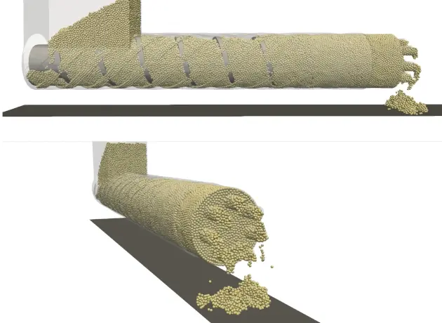
Industrial processes involve millions of particles, complex geometries and long process times, and results are still needed quickly. Aspherix® is built to handle this, from a desktop workstation to a large HPC cluster or the cloud, with no change to the simulation setup. You typically set up the case in the GUI and then send it to the cluster for computation.
On CPUs, standard MPI parallelization has shown near-linear scaling up to 1,000 cores and 100 million particles. Dynamic load balancing keeps all cores busy even when the particles fill only a small, moving part of the domain. On NVIDIA GPUs, a single graphics card matches or beats 64 CPU cores for cases above roughly 500,000 particles. Independent benchmarks found Aspherix® about 3× faster than its predecessor LIGGGHTS® on CPU. This makes industrial-scale simulations practical in everyday engineering work.
Coarse-graining represents groups of particles as larger parcels while keeping the bulk behavior. Scaling laws are applied automatically to contacts, cohesion, drag and heat and mass exchange, so no manual re-tuning is needed. Dynamic coarsening and refinement put detail only where it matters, saving up to 8× in computing effort in a Wurster coater.
Simulation of an industrial scale rotary kiln on an HPC CPU cluster
A simulation is only as valuable as the insight it delivers. Pictures of moving particles are a good start, but process decisions need numbers: How well is the powder mixed? How long does the material stay in the drum? Where are the highest loads on the equipment? Aspherix® answers these questions with evaluations built into the software, set up alongside the simulation in the GUI and calculated while it runs.
Particle data can be averaged in space and time, summarized as mixing indices, mass flows and centers of mass, or evaluated in cross-sections and Voronoi cells. Residence time and residence distance distributions show how material moves through the process. Contact and bond networks, stress tensors and wall loads reveal the forces inside the bulk and on the equipment, while collision statistics and the energy balance explain where energy is put in and dissipated. Steady-state detection tells you when the results are ready to use, and evaluations can also be repeated on finished simulations.
All results are written as CSV and VTK files for graphs and animated playback, including in ParaView with a dedicated Aspherix® macro. This turns raw particle data into answers you can act on.
Visualization of the electric current in the particle contact network
Evaluation of impeller torque and residual solvent content during agitated filter drying
Particles rarely act alone. They are carried by gas flows, load and deform structures, interact with moving machine parts and respond to electric fields. Many of these effects can be modelled directly in Aspherix®, but some need dedicated software. For these, Aspherix® comes with ready-made interfaces to other simulation tools.
With our particle fluid software CFDEM®coupling particles and fluid are fully coupled in both directions, including heat and species transport and reactive multiphase flows. The coupling with the Elmer FEM solver passes particle loads to a structure and sends the resulting deformation back to the DEM simulation. Through the FMI standard, a multibody dynamics code such as Simulink/Simscape or MSC Adams moves the DEM geometries and receives the particle forces and torques in return. Electrostatic forces act on charged particles, with optional charge transfer when they collide.
By combining Aspherix® with these specialised tools, you can simulate the whole process, including flow, structure, machine and field effects, not just the particles.
Fully coupled CFD-DEM simulation to model erosion around a bridge
Aspherix® can do more than run standalone simulations: you can also drive it from your own code. The C++ and Python APIs let you embed the DEM solver in your own applications and workflows, run input files or single commands from a script, and control a simulation step by step. You can read and change particle, contact, mesh and simulation data directly, without going through files.
For special physics, you can add your own contact models and custom commands through the API. This lets you run parameter studies, optimisation loops, use Aspherix® as the DEM part of a larger simulation chain, or connect it to your own tools.
Start testing now.